Data decimation for very large datasets
Both panels plot the same hundred-thousand-sample vibration record. The upper (over its whole time extent) is decimated (points and lines are collapsed where they overlap) for quick rendering and compact export, while retaining significant features in the data. When zoomed in, as in the lower panel, data is rendered in full.
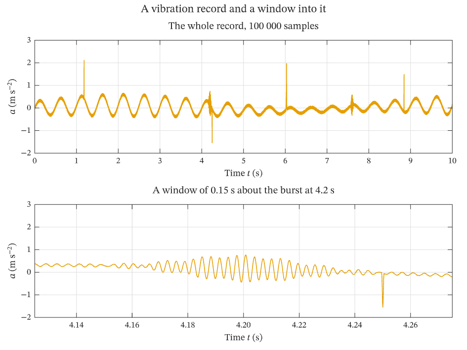
Select the image, or download the PDF, to open the vector figure exported by IronLAB.
Source
The figure is built by the following code.
use std::f64::consts::TAU;

use ironlab::prelude::*;

pub const TITLE: &str = "Data decimation for very large datasets";
pub const DESCRIPTION: &str = "Both panels plot the same hundred-thousand-sample vibration record. The upper (over \
     its whole time extent) is decimated (points and lines are collapsed where they overlap) for quick rendering and compact \
     export, while retaining significant features in the data. When zoomed in, as in the lower panel, data is rendered in \
     full.";

/// The number of samples in the record, which is far more than any plot of it can resolve.
const SAMPLES: usize = 100_000;

/// The duration of the record, in seconds, giving a sampling rate of 10 kHz.
const DURATION_S: f64 = 10.0;

/// The centre of the window shown in the lower panel, in seconds.
const WINDOW_CENTRE_S: f64 = 4.2;

/// The half-width of the window shown in the lower panel, in seconds.
const WINDOW_HALF_WIDTH_S: f64 = 0.075;

/// The frequency of the ripple that rides on the carrier, in hertz.
///
/// It completes 2500 cycles over the record, so the overview can only show its envelope, and 37 cycles over the
/// window, where it is drawn as the oscillation it is.
const RIPPLE_HZ: f64 = 250.0;

/// The centre, peak amplitude and frequency of each burst of ringing: `(seconds, m s⁻², hertz)`.
const BURSTS: [(f64, f64, f64); 2] = [(WINDOW_CENTRE_S, 0.55, 320.0), (7.6, 0.4, 260.0)];

/// The time constant of a burst, in seconds, which decides how quickly its ringing dies away.
const BURST_DECAY_S: f64 = 0.02;

/// The centre time and peak amplitude of each transient: `(seconds, m s⁻²)`.
const TRANSIENTS: [(f64, f64); 4] = [(1.184, 1.7), (4.25, -1.5), (6.031, 2.1), (8.845, 1.6)];

/// The half-width of a transient, in samples: four ten-thousandths of a second, or a third of a pixel in the
/// overview and two points wide in the window.
const TRANSIENT_HALF_WIDTH: usize = 4;

/// Returns the time of sample `i`, in seconds.
fn time_of(i: usize) -> f64 {
    i as f64 * DURATION_S / (SAMPLES - 1) as f64
}

/// Returns a reproducible dither in `[-1, 1]`, from an integer hash of the sample index.
fn dither(i: usize) -> f64 {
    let mixed = (i as u64).wrapping_mul(0x9E37_79B9_7F4A_7C15);
    let mixed = (mixed ^ (mixed >> 31)).wrapping_mul(0xBF58_476D_1CE4_E5B9);
    ((mixed >> 11) as f64) / ((1u64 << 53) as f64) * 2.0 - 1.0
}

/// Returns the ringing of the bursts at time `t`, each a decaying oscillation under a Gaussian envelope.
fn bursts(t: f64) -> f64 {
    BURSTS
        .iter()
        .map(|&(centre_s, amplitude, frequency_hz)| {
            let offset_s = t - centre_s;
            let envelope = (-0.5 * (offset_s / BURST_DECAY_S).powi(2)).exp();
            amplitude * envelope * (TAU * frequency_hz * offset_s).sin()
        })
        .sum()
}

/// Returns the contribution of the transients at sample `i`, each a raised cosine a few samples wide.
fn transients(i: usize) -> f64 {
    TRANSIENTS
        .iter()
        .map(|&(centre_s, amplitude)| {
            let centre = (centre_s / DURATION_S * (SAMPLES - 1) as f64).round() as usize;
            let offset = i.abs_diff(centre);
            if offset >= TRANSIENT_HALF_WIDTH {
                return 0.0;
            }
            let phase = offset as f64 / TRANSIENT_HALF_WIDTH as f64;
            amplitude * 0.5 * (1.0 + (TAU / 2.0 * phase).cos())
        })
        .sum()
}

/// Returns the acceleration at sample `i`, in m s⁻².
///
/// The record has structure at four scales: a slow drift and a beating carrier that the overview shows, a ripple
/// and bursts of ringing that only a narrow window resolves, and transients a few samples wide.
fn acceleration_at(i: usize) -> f64 {
    let t = time_of(i);
    let envelope = 0.30 + 0.18 * (0.7 * t).sin();
    envelope * (TAU * 2.0 * t).sin()
        + 0.12 * (TAU * 0.13 * t).sin()
        + 0.06 * (TAU * RIPPLE_HZ * t).sin()
        + bursts(t)
        + transients(i)
        + 0.008 * dither(i)
}

pub fn figure() -> Figure {
    let t: Vec<f64> = (0..SAMPLES).map(time_of).collect();
    let acceleration: Vec<f64> = (0..SAMPLES).map(acceleration_at).collect();

    let mut fig = Figure::new()
        .size_mm(160.0, 120.0)
        .tiles(2, 1)
        .title("A vibration record and a window into it");

    let mut overview = fig.axes(0, 0);
    overview.plot(&t, &acceleration);
    overview
        .title("The whole record, 100 000 samples")
        .xlabel(r"Time $t$ (s)")
        .ylabel(r"$a$ (m s$^{-2}$)")
        .grid(true);

    // The lower panel plots the same record and differs only in its x limits, so what it adds is detail that the
    // view of the upper panel cannot resolve rather than different data.
    let mut window = fig.axes(1, 0);
    window.plot(&t, &acceleration);
    window
        .title("A window of 0.15 s about the burst at 4.2 s")
        .xlim(
            WINDOW_CENTRE_S - WINDOW_HALF_WIDTH_S,
            WINDOW_CENTRE_S + WINDOW_HALF_WIDTH_S,
        )
        .xlabel(r"Time $t$ (s)")
        .ylabel(r"$a$ (m s$^{-2}$)")
        .grid(true);
    fig
}