Histograms
The diameters of 400 shafts turned on each of two lathes to a nominal 25 mm, drawn from seeded normal distributions: the first lathe is centred on the nominal diameter, and the second, whose tool has worn, cuts 12 µm oversize and spreads its parts more widely. On the left the two samples are binned on the same edges and normalised as probability densities, so that each outline encloses unit area however many shafts it counts, and drawn as step outlines, which overlay without hiding one another. Over each outline is the normal density with the mean and standard deviation of its sample. On the right the same samples are stacked as counts on the same edges, so that the top of each stack is the histogram of the whole production. Each histogram stores its binned values together with a record of how they were binned, so a datatip in the viewer reports the count and density of the bin under the pointer.
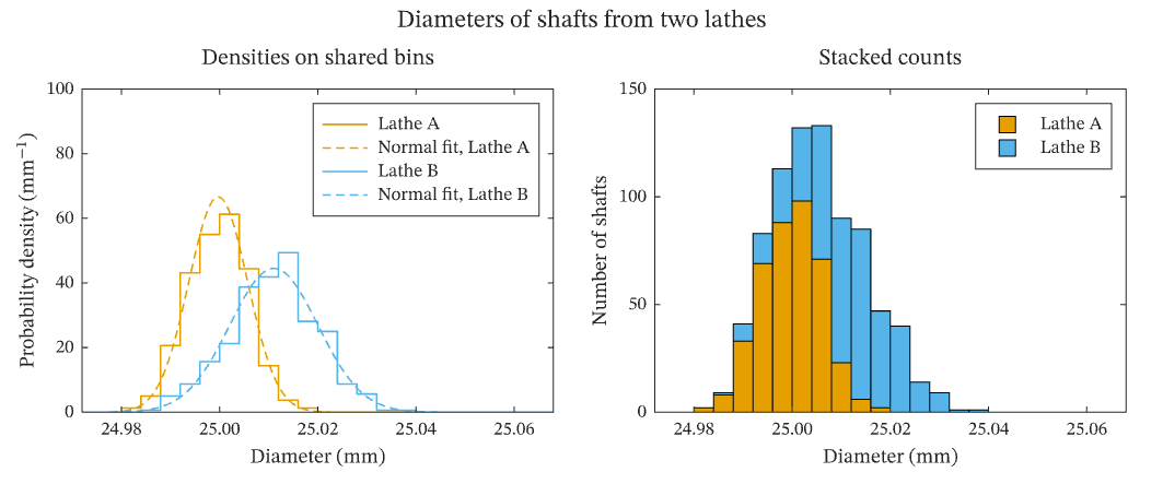
The figure above is live, drawn in the browser by the same engine that draws the viewer: drag it to pan, and click it to zoom with the wheel. Download the PDF for the vector figure that IronLAB exports, or read how to embed a figure of your own.
Source
The figure is built by the following code.
use ironlab::prelude::*;

pub const TITLE: &str = "Histograms";
pub const DESCRIPTION: &str = "The diameters of 400 shafts turned on each of two lathes to a nominal 25 mm, \
     drawn from seeded normal distributions: the first lathe is centred on the nominal diameter, and the second, \
     whose tool has worn, cuts 12 µm oversize and spreads its parts more widely. On the left the two samples are \
     binned on the same edges and normalised as probability densities, so that each outline encloses unit area \
     however many shafts it counts, and drawn as step outlines, which overlay without hiding one another. Over each \
     outline is the normal density with the mean and standard deviation of its sample. On the right the same \
     samples are stacked as counts on the same edges, so that the top of each stack is the histogram of the whole \
     production. Each histogram stores its binned values together with a record of how they were binned, so a \
     datatip in the viewer reports the count and density of the bin under the pointer.";

/// The nominal diameter, in millimetres.
const NOMINAL_MM: f64 = 25.0;

/// The number of shafts turned on each lathe.
const SHAFTS: usize = 400;

/// The lathes: a name, the mean offset of their diameters from the nominal and their standard deviation, in
/// micrometres, and the seed of their sample.
const LATHES: [(&str, f64, f64, u64); 2] = [("Lathe A", 0.0, 6.0, 7), ("Lathe B", 12.0, 9.0, 11)];

/// A small deterministic generator, so that the samples are the same on every run.
struct SplitMix64(u64);

impl SplitMix64 {
    /// Returns a number drawn uniformly from `(0, 1)`.
    fn unit(&mut self) -> f64 {
        self.0 = self.0.wrapping_add(0x9e37_79b9_7f4a_7c15);
        let mut z = self.0;
        z = (z ^ (z >> 30)).wrapping_mul(0xbf58_476d_1ce4_e5b9);
        z = (z ^ (z >> 27)).wrapping_mul(0x94d0_49bb_1331_11eb);
        z ^= z >> 31;
        ((z >> 11) as f64 + 0.5) / (1u64 << 53) as f64
    }

    /// Returns a number drawn from the standard normal distribution, by the Box–Muller transform.
    fn normal(&mut self) -> f64 {
        let (u, v) = (self.unit(), self.unit());
        (-2.0 * u.ln()).sqrt() * (std::f64::consts::TAU * v).cos()
    }
}

/// Returns the diameters, in millimetres, of the shafts of a lathe whose diameters are offset from the nominal by
/// `offset_um` on average, with the standard deviation `sigma_um`.
fn diameters(offset_um: f64, sigma_um: f64, seed: u64) -> Vec<f64> {
    let mut rng = SplitMix64(seed);
    (0..SHAFTS)
        .map(|_| NOMINAL_MM + 1.0e-3 * (offset_um + sigma_um * rng.normal()))
        .collect()
}

/// Returns the mean and the standard deviation of a sample.
fn mean_and_deviation(sample: &[f64]) -> (f64, f64) {
    let n = sample.len() as f64;
    let mean = sample.iter().sum::<f64>() / n;
    let variance = sample.iter().map(|x| (x - mean).powi(2)).sum::<f64>() / (n - 1.0);
    (mean, variance.sqrt())
}

pub fn figure() -> Figure {
    let samples: Vec<Vec<f64>> = LATHES
        .iter()
        .map(|&(_, offset, sigma, seed)| diameters(offset, sigma, seed))
        .collect();
    // Shared bins 4 µm wide, wide enough to hold every shaft of both lathes.
    let edges: Vec<f64> = (0..=24).map(|k| NOMINAL_MM - 0.028 + 0.004 * f64::from(k)).collect();
    let x = linspace(edges[0], edges[edges.len() - 1], 201);

    let mut fig = Figure::new()
        .size_mm(180.0, 75.0)
        .tiles(1, 2)
        .title("Diameters of shafts from two lathes")
        .tag("bar")
        .tag("stairs")
        .tag("line")
        .tag("subplots")
        .tag("legend")
        .tag("statistics")
        .tag("measurements")
        .tag("comparison")
        .tag("histogram")
        .tag("density")
        .tag("stacked")
        .tag("distribution")
        .parameter("dimensionality", "2D")
        .parameter("artists", 6)
        .parameter("data_points", 1071)
        .parameter("has_legend", true);

    let mut ax = fig.axes(0, 0);
    // The first two colours of the colour order, which the stacked histograms on the right take automatically, so
    // that each lathe has one colour in both axes and its fitted density is drawn in that colour too.
    let colors = [Color::rgb(0.902, 0.624, 0.0), Color::rgb(0.337, 0.706, 0.914)];
    for ((sample, &(name, ..)), color) in samples.iter().zip(&LATHES).zip(colors) {
        ax.hist(sample)
            .bins(Bins::Edges(edges.clone()))
            .normalize(HistNorm::Density)
            .style(HistStyle::Step)
            .color(color)
            .label(name);
        let (mean, sigma) = mean_and_deviation(sample);
        let pdf: Vec<f64> = x
            .iter()
            .map(|x| {
                (-0.5 * ((x - mean) / sigma).powi(2)).exp()
                    / (sigma * std::f64::consts::TAU.sqrt())
            })
            .collect();
        ax.plot(&x, &pdf)
            .label(format!("Normal fit, {name}"))
            .color(color)
            .dash(Dash::Dashed);
    }
    ax.xlim(edges[0], edges[edges.len() - 1])
        .ylim(0.0, 100.0)
        .xlabel("Diameter (mm)")
        .ylabel(r"Probability density (mm$^{-1}$)")
        .title("Densities on shared bins")
        .legend(LegendLocation::NorthEast);

    let mut ax = fig.axes(0, 1);
    let mut stack = ax.hists(Bins::Edges(edges.clone()));
    for (sample, &(name, ..)) in samples.iter().zip(&LATHES) {
        stack.stacked("production", name, sample);
    }
    ax.xlim(edges[0], edges[edges.len() - 1])
        .xlabel("Diameter (mm)")
        .ylabel("Number of shafts")
        .title("Stacked counts")
        .legend(LegendLocation::NorthEast);
    fig
}