Two-dimensional histogram and density contour
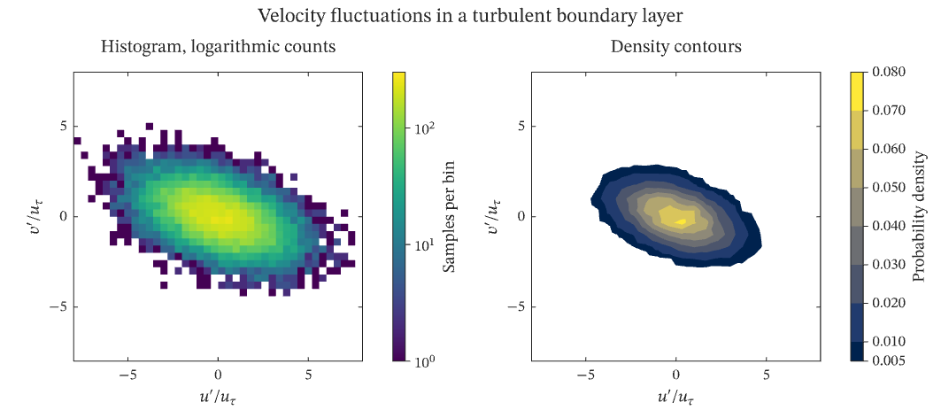
The joint distribution of the streamwise and wall-normal velocity fluctuations u′ and v′ in the logarithmic region of a turbulent boundary layer, scaled by the friction velocity, as 20 000 seeded samples of a correlated normal distribution. The fluctuations are anticorrelated: fluid moving away from the wall is slower than the mean, and fluid moving towards it faster, which is the Reynolds shear stress −u′v′ that carries momentum to the wall. On the left the pairs are binned on a 40 × 40 grid and drawn as cells coloured by their count through a logarithmic colour scale; bins with no sample are left empty, because a logarithmic scale cannot place a count of zero. On the right the same samples are binned more coarsely and drawn as filled contours of their probability density, banded by a discrete colour scale whose lowest edge lies above zero and which draws nothing below it, so that the plane where no sample lies stays blank. Each scale is shown by a colourbar in the fitted column beside its axes, and both axes are drawn at equal aspect, so that the tilt of the distribution reads true.
The figure above is live, drawn in the browser by the same engine that draws the viewer: drag it to pan, and click it to zoom with the wheel. Download the PDF for the vector figure that IronLAB exports, or read how to embed a figure of your own.
Source
The figure is built by the following code.
use ironlab::prelude::*;

pub const TITLE: &str = "Two-dimensional histogram and density contour";
pub const DESCRIPTION: &str = "The joint distribution of the streamwise and wall-normal velocity fluctuations u′ \
     and v′ in the logarithmic region of a turbulent boundary layer, scaled by the friction velocity, as 20 000 \
     seeded samples of a correlated normal distribution. The fluctuations are anticorrelated: fluid moving away from \
     the wall is slower than the mean, and fluid moving towards it faster, which is the Reynolds shear stress −u′v′ \
     that carries momentum to the wall. On the left the pairs are binned on a 40 × 40 grid and drawn as cells \
     coloured by their count through a logarithmic colour scale; bins with no sample are left empty, because a \
     logarithmic scale cannot place a count of zero. On the right the same samples are binned more coarsely and \
     drawn as filled contours of their probability density, banded by a discrete colour scale whose lowest edge lies \
     above zero and which draws nothing below it, so that the plane where no sample lies stays blank. Each scale is \
     shown by a colourbar in the fitted column beside its axes, and both axes are drawn at equal aspect, so that the \
     tilt of the distribution reads true.";

/// The number of samples.
const SAMPLES: usize = 20_000;

/// The standard deviations of u′ and v′ and their correlation coefficient.
const U_RMS: f64 = 2.0;
const V_RMS: f64 = 1.2;
const CORRELATION: f64 = -0.45;

/// The limits of both velocity axes, in units of the friction velocity.
const LIMIT: f64 = 8.0;

/// A small deterministic generator, so that the samples are the same on every run.
struct SplitMix64(u64);

impl SplitMix64 {
    /// Returns a number drawn uniformly from `(0, 1)`.
    fn unit(&mut self) -> f64 {
        self.0 = self.0.wrapping_add(0x9e37_79b9_7f4a_7c15);
        let mut z = self.0;
        z = (z ^ (z >> 30)).wrapping_mul(0xbf58_476d_1ce4_e5b9);
        z = (z ^ (z >> 27)).wrapping_mul(0x94d0_49bb_1331_11eb);
        z ^= z >> 31;
        ((z >> 11) as f64 + 0.5) / (1u64 << 53) as f64
    }

    /// Returns a pair of independent numbers drawn from the standard normal distribution, by the Box–Muller
    /// transform.
    fn normal_pair(&mut self) -> (f64, f64) {
        let (u, v) = (self.unit(), self.unit());
        let radius = (-2.0 * u.ln()).sqrt();
        let angle = std::f64::consts::TAU * v;
        (radius * angle.cos(), radius * angle.sin())
    }
}

/// Returns the samples of u′ and v′, correlated by mixing two independent normal samples.
fn fluctuations() -> (Vec<f64>, Vec<f64>) {
    let mut rng = SplitMix64(2026);
    let mixing = (1.0 - CORRELATION * CORRELATION).sqrt();
    (0..SAMPLES)
        .map(|_| {
            let (a, b) = rng.normal_pair();
            (U_RMS * a, V_RMS * (CORRELATION * a + mixing * b))
        })
        .unzip()
}

pub fn figure() -> Figure {
    let (u, v) = fluctuations();

    let mut fig = Figure::new()
        .size_mm(180.0, 80.0)
        .tiles(1, 4)
        .fit_col(1)
        .fit_col(3)
        .title("Velocity fluctuations in a turbulent boundary layer")
        .tag("cells")
        .tag("contour")
        .tag("subplots")
        .tag("color-scale")
        .tag("colorbar")
        .tag("aspect")
        .tag("statistics")
        .tag("histogram")
        .tag("2d-histogram")
        .tag("density")
        .tag("turbulence")
        .parameter("dimensionality", "2D")
        .parameter("artists", 2)
        .parameter("data_points", 2306)
        .parameter("has_legend", false);

    let mut ax = fig.axes(0, 0);
    ax.hist2d(&u, &v)
        .bins(Bins::Count(40), Bins::Count(40))
        .range((-LIMIT, LIMIT), (-LIMIT, LIMIT))
        .min_count(1.0);
    let counts = ax
        .color_scale()
        .norm(ColorScaleNorm::Log)
        .limits(1.0, 300.0)
        .ticks([1.0, 10.0, 100.0])
        .title("Samples per bin")
        .id();
    ax.xlim(-LIMIT, LIMIT)
        .ylim(-LIMIT, LIMIT)
        .aspect(Aspect::Equal)
        .xlabel(r"$u'/u_\tau$")
        .ylabel(r"$v'/u_\tau$")
        .title("Histogram, logarithmic counts");
    fig.panel(0, 1).colorbar(counts);

    // The density is banded by a discrete scale whose lowest edge is above zero and which draws nothing below it,
    // so that the contours show where the samples lie and leave the empty plane blank. The filled contour has no
    // levels of its own and takes the band edges of the scale.
    let density = fig
        .color_scale()
        .colormap(Colormap::Cividis)
        .discrete([0.005, 0.01, 0.02, 0.03, 0.04, 0.05, 0.06, 0.07, 0.08])
        .below(OutOfRange::Transparent)
        .title("Probability density")
        .id();
    let mut ax = fig.axes(0, 2);
    ax.density_contour(&u, &v)
        .bins(Bins::Count(24), Bins::Count(24))
        .range((-LIMIT, LIMIT), (-LIMIT, LIMIT))
        .normalize(HistNorm::Density)
        .filled(true)
        .color_scale(density);
    ax.xlim(-LIMIT, LIMIT)
        .ylim(-LIMIT, LIMIT)
        .aspect(Aspect::Equal)
        .xlabel(r"$u'/u_\tau$")
        .ylabel(r"$v'/u_\tau$")
        .title("Density contours");
    fig.panel(0, 3).colorbar(density);
    fig
}