Logarithmic axes
Power laws on log-log axes, the magnitude response of a low-pass filter on a logarithmic frequency axis, and exponential decays on a logarithmic vertical axis.
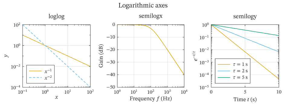
Select the image, or download the PDF, to open the vector figure exported by IronLAB.
Source
The figure is built by the following code.
use ironlab::prelude::*;

pub const TITLE: &str = "Logarithmic axes";
pub const DESCRIPTION: &str = "Power laws on log-log axes, the magnitude response of a low-pass filter on a \
     logarithmic frequency axis, and exponential decays on a logarithmic vertical axis.";

pub fn figure() -> Figure {
    let mut fig = Figure::new()
        .size_mm(160.0, 60.0)
        .tiles(1, 3)
        .title("Logarithmic axes");

    // Power laws are straight lines on log-log axes, with slopes equal to their exponents.
    let x = logspace(-1.0, 2.0, 61);
    let inverse: Vec<f64> = x.iter().map(|x| 1.0 / x).collect();
    let inverse_square: Vec<f64> = x.iter().map(|x| 1.0 / (x * x)).collect();
    let mut ax = fig.axes(0, 0);
    ax.loglog(&x, &inverse).display_name("$x^{-1}$");
    ax.loglog(&x, &inverse_square)
        .display_name("$x^{-2}$")
        .dash(Dash::Dashed);
    ax.title("loglog")
        .xlabel("$x$")
        .ylabel("$y$")
        .grid(true)
        .legend(LegendLocation::SouthWest);

    // A first-order low-pass filter loses 20 dB per decade above its cut-off frequency.
    let cutoff_hz = 100.0;
    let frequency_hz = logspace(0.0, 4.0, 81);
    let gain_db: Vec<f64> = frequency_hz
        .iter()
        .map(|f| -10.0 * (1.0 + (f / cutoff_hz).powi(2)).log10())
        .collect();
    let mut ax = fig.axes(0, 1);
    ax.semilogx(&frequency_hz, &gain_db);
    ax.title("semilogx")
        .xlabel("Frequency $f$ (Hz)")
        .ylabel("Gain (dB)")
        .grid(true);

    // Exponential decays are straight lines when only the vertical axis is logarithmic.
    let t = linspace(0.0, 10.0, 51);
    let mut ax = fig.axes(0, 2);
    for tau in [1.0, 2.0, 5.0] {
        // tau is the time constant in seconds.
        let decay: Vec<f64> = t.iter().map(|t| (-t / tau).exp()).collect();
        ax.semilogy(&t, &decay)
            .display_name(format!(r"$\tau = {tau}$ s"));
    }
    ax.title("semilogy")
        .xlabel("Time $t$ (s)")
        .ylabel(r"$e^{-t/\tau}$")
        .grid(true)
        .legend(LegendLocation::SouthWest);

    fig
}