Logarithmic colour scale
The ground-level concentration of a pollutant downwind of a 60 m stack, from the Gaussian plume model with the Briggs dispersion coefficients of a neutral atmosphere. The concentration spans four decades over the plume, so the scalar image maps it through a colour scale with a logarithmic norm between 0.1 and 1000 µg/m³, which gives each decade an equal share of the colormap. The scale draws nothing for a concentration below 0.1 µg/m³, so the air the plume has not reached is left blank rather than painted in the first colour, and the black isolines mark the decades 0.1, 1, 10 and 100 µg/m³. The colourbar beside the axes is ticked at the decades, which are equally spaced along it, and its empty key below the bar stands for the concentrations below 0.1 µg/m³ that are left blank.
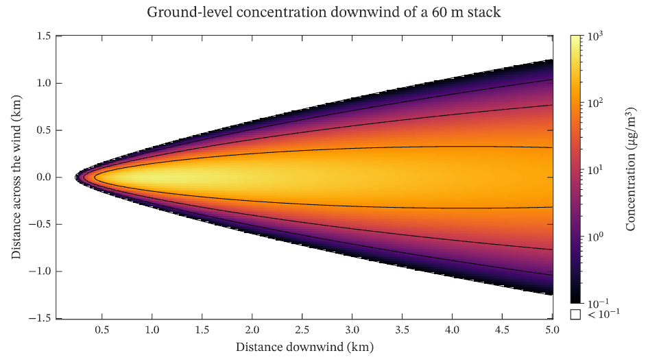
The figure above is live, drawn in the browser by the same engine that draws the viewer: drag it to pan, and click it to zoom with the wheel. Download the PDF for the vector figure that IronLAB exports, or read how to embed a figure of your own.
Source
The figure is built by the following code.
use ironlab::prelude::*;

pub const TITLE: &str = "Logarithmic colour scale";
pub const DESCRIPTION: &str = "The ground-level concentration of a pollutant downwind of a 60 m stack, from the \
     Gaussian plume model with the Briggs dispersion coefficients of a neutral atmosphere. The concentration spans \
     four decades over the plume, so the scalar image maps it through a colour scale with a logarithmic norm between \
     0.1 and 1000 µg/m³, which gives each decade an equal share of the colormap. The scale draws nothing for a \
     concentration below 0.1 µg/m³, so the air the plume has not reached is left blank rather than painted in the \
     first colour, and the black isolines mark the decades 0.1, 1, 10 and 100 µg/m³. The colourbar beside the axes \
     is ticked at the decades, which are equally spaced along it, and its empty key below the bar stands for the \
     concentrations below 0.1 µg/m³ that are left blank.";

/// The emission rate of the stack, in grams per second.
const EMISSION_G_PER_S: f64 = 100.0;

/// The wind speed at the height of the stack, in metres per second.
const WIND_M_PER_S: f64 = 5.0;

/// The effective height of the stack, in metres.
const STACK_HEIGHT_M: f64 = 60.0;

/// The number of samples downwind of the stack.
const DOWNWIND: usize = 251;

/// The number of samples across the wind.
const CROSSWIND: usize = 151;

/// Returns the ground-level concentration, in micrograms per cubic metre, at a distance `x` downwind of the stack and
/// `y` across the wind, both in metres, from the Gaussian plume model with reflection at the ground.
///
/// The lateral and vertical spreads are the Briggs coefficients for open country in a neutral atmosphere (Pasquill
/// class D), σy = 0.08 x (1 + 0.0001 x)^−½ and σz = 0.06 x (1 + 0.0015 x)^−½.
fn concentration(x: f64, y: f64) -> f64 {
    let sigma_y = 0.08 * x / (1.0 + 0.0001 * x).sqrt();
    let sigma_z = 0.06 * x / (1.0 + 0.0015 * x).sqrt();
    let grams_per_m3 = EMISSION_G_PER_S / (std::f64::consts::PI * WIND_M_PER_S * sigma_y * sigma_z)
        * (-y * y / (2.0 * sigma_y * sigma_y)).exp()
        * (-STACK_HEIGHT_M * STACK_HEIGHT_M / (2.0 * sigma_z * sigma_z)).exp();
    grams_per_m3 * 1e6
}

pub fn figure() -> Figure {
    let x_km = linspace(0.05, 5.0, DOWNWIND);
    let y_km = linspace(-1.5, 1.5, CROSSWIND);
    let c = Matrix::from_fn(CROSSWIND, DOWNWIND, |row, col| {
        concentration(x_km[col] * 1000.0, y_km[row] * 1000.0)
    });

    let mut fig = Figure::new()
        .size_mm(160.0, 90.0)
        .tiles(1, 2)
        .fit_col(1)
        .title("Ground-level concentration downwind of a 60 m stack")
        .tag("image")
        .tag("contour")
        .tag("color-scale")
        .tag("out-of-range")
        .tag("colorbar")
        .parameter("dimensionality", "2D")
        .parameter("artists", 2)
        .parameter("data_points", 38_303)
        .parameter("has_legend", false);
    let c = fig.data("concentration (µg/m³)", c).id();
    let decades = fig
        .color_scale()
        .colormap(Colormap::Inferno)
        .norm(ColorScaleNorm::Log)
        .limits(0.1, 1000.0)
        .below(OutOfRange::Transparent)
        .show_key(ColorScaleKey::Below)
        .title("Concentration (µg/m³)")
        .id();

    let mut ax = fig.axes(0, 0);
    ax.scalar_image(c)
        .pixel_columns(x_km[0], x_km[DOWNWIND - 1])
        .pixel_rows(y_km[0], y_km[CROSSWIND - 1])
        .color_scale(decades);
    ax.contour(&x_km, &y_km, c)
        .level_values([0.1, 1.0, 10.0, 100.0])
        .color(Color::BLACK)
        .line_width(0.5);
    ax.xlabel("Distance downwind (km)")
        .ylabel("Distance across the wind (km)");
    fig.panel(0, 1).colorbar(decades);
    fig
}