Wide legend panel
The step response and the magnitude response of a second-order system for twelve damping ratios, with one legend panel spanning the full width of the figure below both plots. The panel arranges its twelve entries in as few columns as fit its height, and the rows of tiles are weighted 3 : 1 so that the panel is a third as tall as the plots above it.
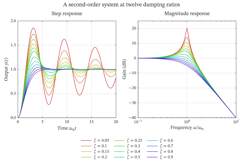
The figure above is live, drawn in the browser by the same engine that draws the viewer: drag it to pan, and click it to zoom with the wheel. Download the PDF for the vector figure that IronLAB exports, or read how to embed a figure of your own.
Source
The figure is built by the following code. Its data comes from the functions on the data helpers page.
use ironlab::prelude::*;

use crate::fields::hsl_to_rgb;

pub const TITLE: &str = "Wide legend panel";
pub const DESCRIPTION: &str = "The step response and the magnitude response of a second-order system for twelve \
     damping ratios, with one legend panel spanning the full width of the figure below both plots. The panel \
     arranges its twelve entries in as few columns as fit its height, and the rows of tiles are weighted 3 : 1 so \
     that the panel is a third as tall as the plots above it.";

const DAMPING_RATIOS: [f64; 12] = [
    0.05, 0.1, 0.15, 0.2, 0.25, 0.3, 0.4, 0.5, 0.6, 0.7, 0.8, 0.9,
];

/// Returns the unit step response at time `t` of an underdamped second-order system with a natural frequency of
/// 1 rad/s and damping ratio `zeta`.
fn step_response(t: f64, zeta: f64) -> f64 {
    let damped = (1.0 - zeta * zeta).sqrt();
    1.0 - (-zeta * t).exp() * ((damped * t).cos() + zeta / damped * (damped * t).sin())
}

/// Returns the gain in decibels at angular frequency `omega` of the same system.
fn gain_db(omega: f64, zeta: f64) -> f64 {
    -10.0 * ((1.0 - omega * omega).powi(2) + (2.0 * zeta * omega).powi(2)).log10()
}

pub fn figure() -> Figure {
    let t = linspace(0.0, 20.0, 201);
    let omega = logspace(-1.0, 1.0, 201);

    let mut fig = Figure::new()
        .size_mm(160.0, 110.0)
        .tiles(2, 2)
        .row_weights([3.0, 1.0])
        .title("A second-order system at twelve damping ratios")
        .tag("line")
        .tag("subplots")
        .tag("legend")
        .tag("log")
        .tag("signals")
        .parameter("dimensionality", "2D")
        .parameter("artists", 24)
        .parameter("data_points", 9648)
        .parameter("has_legend", true);
    // A full-width panel in the bottom row, drawn without the border a panel has by default; its default automatic
    // columns spread the entries across its width.
    let key = fig.panel_span(1, 0, 1, 2).legend().boxed(false).id();

    for (k, &zeta) in DAMPING_RATIOS.iter().enumerate() {
        // The lightly damped responses are red and the heavily damped ones violet.
        let color = hsl_to_rgb(0.75 * k as f64 / 11.0, 0.7, 0.45);
        let name = format!(r"$\zeta = {zeta}$");
        let response: Vec<f64> = t.iter().map(|&t| step_response(t, zeta)).collect();
        let gain: Vec<f64> = omega.iter().map(|&omega| gain_db(omega, zeta)).collect();
        fig.axes(0, 0)
            .plot(&t, &response)
            .label(name.as_str())
            .color(color);
        fig.axes(0, 1)
            .semilogx(&omega, &gain)
            .label(name.as_str())
            .color(color);
    }

    fig.axes(0, 0)
        .title("Step response")
        .xlabel(r"Time $\omega_n t$")
        .ylabel("Output $y(t)$")
        .xlim(0.0, 20.0)
        .grid(true)
        .legend_in(key);
    fig.axes(0, 1)
        .title("Magnitude response")
        .xlabel(r"Frequency $\omega / \omega_n$")
        .ylabel("Gain (dB)")
        .ylim(-40.0, 25.0)
        .grid(true)
        .legend_in(key);
    fig
}