Spectrogram on a logarithmic frequency axis
The spectrogram of an exponential sine sweep from 20 Hz to 20 kHz played through a loudspeaker that adds harmonic distortion, as in an acoustic measurement. The sweep rises by the same number of decades every second, so on a logarithmic frequency axis it is a straight line, and its second, third and fourth harmonics are parallel lines above it. The power is drawn as a surface in a two-dimensional axes, whose nodes are placed through the logarithmic scale. An image could not be drawn here: a raster of evenly spaced pixels has no placement on a logarithmic axis, and validation refuses an image whose plane has one.
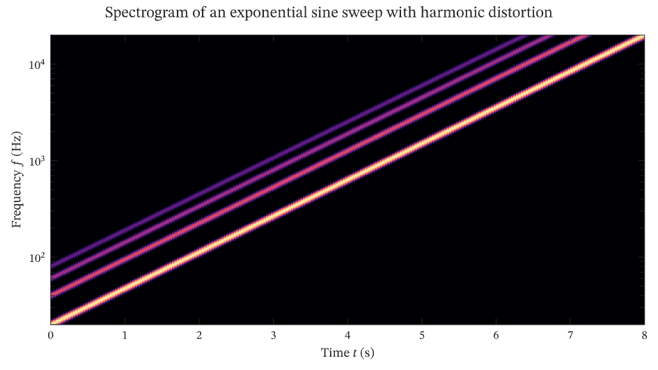
The figure above is live, drawn in the browser by the same engine that draws the viewer: drag it to pan, and click it to zoom with the wheel. Download the PDF for the vector figure that IronLAB exports, or read how to embed a figure of your own.
Source
The figure is built by the following code.
use ironlab::prelude::*;

pub const TITLE: &str = "Spectrogram on a logarithmic frequency axis";
pub const DESCRIPTION: &str = "The spectrogram of an exponential sine sweep from 20 Hz to 20 kHz played through a \
     loudspeaker that adds harmonic distortion, as in an acoustic measurement. The sweep rises by the same number \
     of decades every second, so on a logarithmic frequency axis it is a straight line, and its second, third and \
     fourth harmonics are parallel lines above it. The power is drawn as a surface in a two-dimensional axes, whose \
     nodes are placed through the logarithmic scale. An image could not be drawn here: a raster of evenly spaced \
     pixels has no placement on a logarithmic axis, and validation refuses an image whose plane has one.";

/// The duration of the sweep in seconds.
const DURATION_S: f64 = 8.0;

/// The frequencies at which the sweep starts and ends, in hertz.
const START_HZ: f64 = 20.0;
const END_HZ: f64 = 20_000.0;

/// The power of each harmonic relative to the fundamental, in decibels, starting with the fundamental itself.
const HARMONICS_DB: [f64; 4] = [0.0, -25.0, -35.0, -45.0];

/// The relative bandwidth of the analysis: a constant-Q analysis resolves a tone into a peak whose standard
/// deviation is a fixed fraction of its frequency.
const RELATIVE_BANDWIDTH: f64 = 0.02;

/// The noise floor of the measurement, in decibels relative to the fundamental.
const NOISE_FLOOR_DB: f64 = -70.0;

/// The frequency of the sweep at time `t` in seconds: it rises exponentially, by the same ratio every second.
fn sweep_hz(t: f64) -> f64 {
    START_HZ * (END_HZ / START_HZ).powf(t / DURATION_S)
}

/// The power at time `t` in seconds and frequency `f` in hertz, in decibels relative to the fundamental: a peak at
/// each harmonic of the sweep above the noise floor.
fn power_db(t: f64, f: f64) -> f64 {
    let fundamental = sweep_hz(t);
    let tones: f64 = HARMONICS_DB
        .iter()
        .enumerate()
        .map(|(k, level_db)| {
            let centre = (k + 1) as f64 * fundamental;
            let sigma = RELATIVE_BANDWIDTH * centre;
            10f64.powf(level_db / 10.0) * (-0.5 * ((f - centre) / sigma).powi(2)).exp()
        })
        .sum();
    10.0 * (tones + 10f64.powf(NOISE_FLOOR_DB / 10.0)).log10()
}

pub fn figure() -> Figure {
    // The analysis is evaluated 30 times a second and at frequencies spaced evenly in their logarithm, 80 to a
    // decade.
    let time_s = linspace(0.0, DURATION_S, 241);
    let frequency_hz = logspace(START_HZ.log10(), END_HZ.log10(), 241);
    let power = Matrix::from_fn(frequency_hz.len(), time_s.len(), |row, col| {
        power_db(time_s[col], frequency_hz[row])
    });

    let mut fig = Figure::new()
        .size_mm(160.0, 90.0)
        .title("Spectrogram of an exponential sine sweep with harmonic distortion")
        .tag("surface")
        .tag("log")
        .tag("pcolor")
        .tag("signals")
        .tag("spectrogram")
        .parameter("dimensionality", "2D")
        .parameter("artists", 1)
        .parameter("data_points", 58_563)
        .parameter("has_legend", false);
    let mut ax = fig.axes(0, 0);
    // A surface in a two-dimensional axes is a pseudocolour plot. Its field belongs to the nodes of the grid, which
    // the logarithmic frequency axis places one by one, so the faces between them are as tall as the spacing of the
    // analysis frequencies makes them.
    ax.surface(&time_s, &frequency_hz, &power).edge_color(None);
    ax.color_scale()
        .colormap(Colormap::Magma)
        .limits(NOISE_FLOOR_DB, 0.0);
    ax.yscale(Scale::Log)
        .xlabel("Time $t$ (s)")
        .ylabel("Frequency $f$ (Hz)");
    fig
}